Why a strict quadratic model instead of a hyperbolic fit?

The hyperbolic (Langmuir) form assumes free ligand concentration equals total added concentration. That assumption breaks down once the fixed component's concentration approaches Kd — a regime routine aptamer titrations often sit in. The quadratic equation solves for bound complex explicitly and stays correct under ligand depletion.

Which component should I enter as X, and which as fixed?

X is the component you titrate — the one whose concentration varies across your data rows. fixed is the total concentration of the component held constant in every well or cuvette. The model is symmetric in the two binding partners, so the assignment follows your experiment, not the chemistry.

Should I report the free-Ybase fit or the fixed-Ybase fit?

Report the fixed-Ybase fit when you have independently measured the background — a buffer-only blank, for example. Use the free fit when the baseline is genuinely unknown. The tool runs both on the same dataset precisely so you can see how much the Kd estimate depends on that choice; a large gap between the two is itself a signal that the data underdetermine the baseline.

How many replicates do I need for error bars?

Replicate mode computes sample variance from n ≥ 2 replicates at the same X value. Two replicates will produce error bars, but the variance estimate from n = 2 is very noisy; three or more per concentration gives a bar you can actually interpret.

Is my data uploaded anywhere?

No. Paste handling, fitting, curve sampling and image rendering all run in client-side JavaScript. The page calls no backend, and once it has loaded you can disconnect from the network and keep working.

Tool · Web · No installation

K_d Fitting Tool

Quadratic binding-model K_d fitting from concentration/signal data. Runs entirely in your browser — paste from Excel, fit, export the curve and image. Your data is never uploaded.

Launch K_d Fitting Tool v0.22 · Opens in a new tab See how to use it ↓ 4 steps · ~2 min read

100% browser-local · No account, no upload

/ Introduction

What it does.

K_d Fitting Tool performs nonlinear fitting on the relationship between experimental concentration X and observed signal Y, using the strict quadratic binding equation, to obtain the dissociation constant K_d that best explains the data. The fit is run twice in parallel — once with the baseline Ybase as a free parameter, and once with Ybase fixed to a user-supplied value — so you can compare both interpretations on the same dataset.

Model

Y = Ybase + alpha · [AT]

[AT] = 0.5 · (X + fixed + K_d − √((X + fixed + K_d)² − 4 · X · fixed))

X      = total concentration of the variable component
fixed  = total concentration of the fixed component
K_d     = dissociation constant

Y free fit — Ybase is fitted as a free parameter; the background floats for the best overall fit.

Y fixed fit — Ybase is held at the value you enter; useful when the baseline is independently known.

Strict quadratic model

Uses the full binding equation rather than a simplified hyperbolic approximation — accurate even when ligand depletion matters.
Paste from Excel

Spreadsheet-style table accepts 2- or 3-column paste (X, Y, optional Var(Y)). Replicate mode auto-computes error bars from n ≥ 2 replicates per X.
Error bars, two ways

Manual variance column or replicate-based sample variance — both render error bars on the fitted curve and propagate into the displayed metrics.
Export curve & image

Export the fitted curve as CSV (default 1000 sampled points), or as a PNG / JPG at your chosen PPI for slides and figures.
Side-by-side fit results

Both Y-free and Y-fixed fits run on every click — see K_d, Ybase, alpha, and goodness metrics side by side instead of toggling modes.
Browser-only, zero install

Pure HTML/JS — no plugin, no upload, no account. Works offline once the page is loaded.

/ Usage

How to use it.

Open the tool, paste your data, click Fit. Sample data is loaded by default so you can verify the workflow before entering your own measurements.

01

Open the tool

Click Launch K_d Fitting Tool at the top of this page — it opens in a new tab. The page is self-contained: bookmark it, save it offline, or even open the local HTML file directly.

Screenshot · 01-full-tool.png

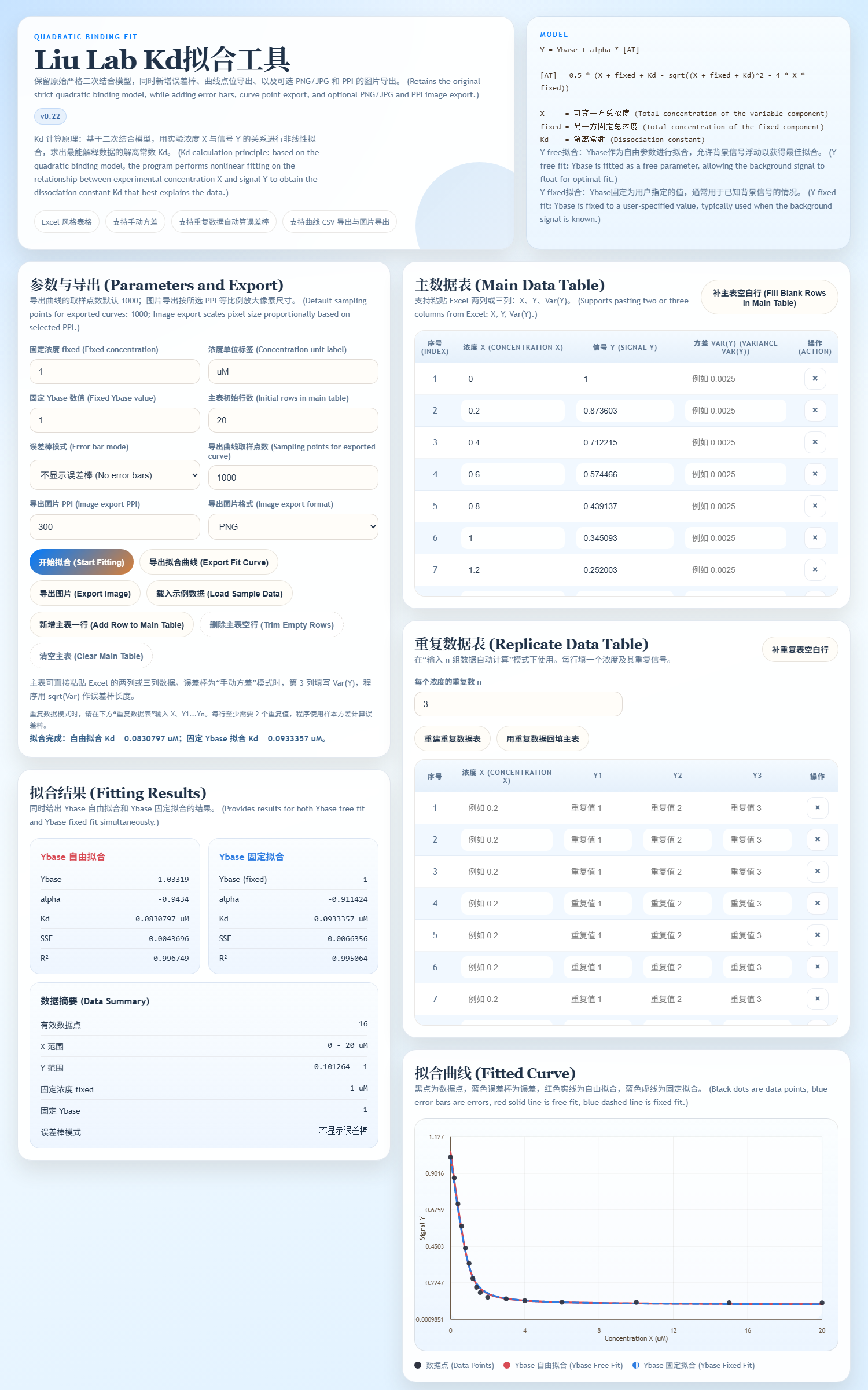
Fig. 01 — Main view
02

Enter parameters

In the Parameters and Export panel, set Fixed concentration (the constant component's total concentration), the unit label (default uM), the fixed Ybase value, and the error-bar mode: None, Manual variance, or Auto from n replicates.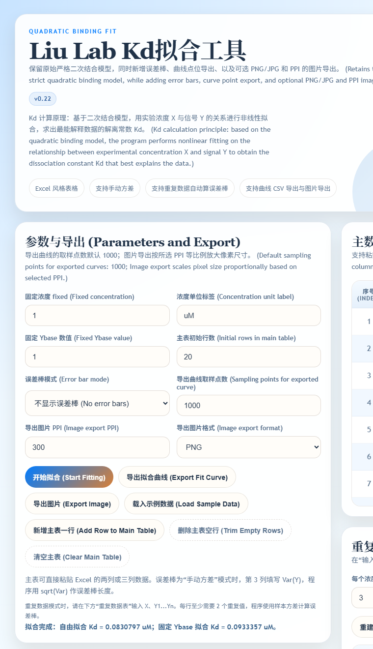

Screenshot · 02-parameters.png

Fig. 02 — Parameter panel
03

Paste your data

In the Main Data Table, paste 2 or 3 columns directly from Excel: X, Y, and optionally Var(Y). For replicate-mode error bars, use the lower Replicate Data Table and enter X, Y₁, Y₂, ... — the program needs at least 2 values per X.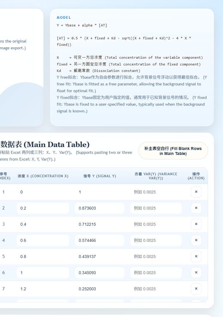

Screenshot · 03-data-table.png

Fig. 03 — Main data table
04

Fit & export

Click Start Fitting. The results panel shows Y-free and Y-fixed fits side by side with K_d, Ybase, alpha, and goodness metrics. The fitted curve appears with your data points; export it as CSV (default 1000 sampled points) or as PNG / JPG at your chosen PPI.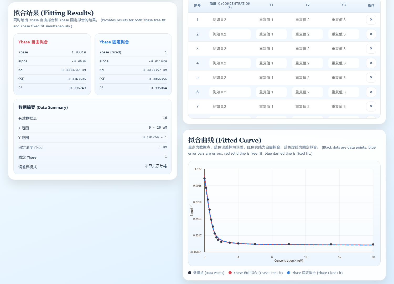

Screenshot · 04-fit-result.png

Fig. 04 — Fit result & curve

/ Disclaimer

Things to know.

Your data never leaves the browser.

All computation — paste handling, fitting, curve sampling, image rendering — runs in client-side JavaScript. Nothing is uploaded; the page does not call any backend.
Works offline once loaded.

The page is fully self-contained: no external scripts, no CDN. After the page loads once, you can disconnect from the network and keep using it. Save the HTML file locally for permanent offline access.
Free for academic / non-commercial use.

K_d Fitting Tool is provided free for academic research and teaching. For commercial integration or redistribution, contact the author in advance.
Provided as-is, without warranty.

Fits are best-effort and depend on data quality. Validate critical results with independent fits (GraphPad, Origin, custom Python) and consider biological/experimental context. Bug reports: [email protected].
Cite if used in publications.

If this tool contributed to a published study, please cite: Zhang X. K_d Fitting Tool, v0.23, Liu Lab, University of Waterloo, 2026. aptapilot.com/tools/kd-fit.

/ Acknowledgments

Built with the lab.

Developed in the Bionanotechnology & Interfaces Laboratory at the University of Waterloo, led by Prof. Juewen Liu. The tool grew out of routine K_d-fitting needs across the group's aptamer / DNAzyme / nanomaterial-binding projects — a thin, accurate, offline-safe alternative to spreadsheet macros and proprietary fitting software.

Prof. Juewen Liu

Advisor

Professor of Chemistry at the University of Waterloo, College member of the Royal Society of Canada (RSC), and Tier 1 Canada Research Chair in Biosensors & Bionanotechnology. Group lead for the aptamer / DNAzyme / nanomaterial research that motivates this tool.
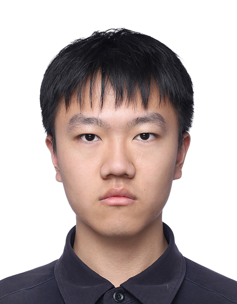
Yuanli Li

Formula development & research

Third-year undergraduate in the Materials Nanoscience joint program (Beijing Jiaotong University × University of Waterloo). Derived and validated the quadratic-binding fit, the Y-free / Y-fixed parameterization, and the replicate-mode variance handling.
Xiaohan Zhang

Web build, visualization & QA

Postdoctoral researcher at the University of Waterloo under Prof. Juewen Liu. Turned the fitting model into a self-contained browser tool — UI, plotting, paste-from-Excel, CSV / PNG export — and ran the cross-dataset QA.

Special thanks to Prof. Bing Jin for guidance and discussion on the binding model.

/ FAQ

Questions people actually ask.

Worked example

A fluorescence titration of a fixed 50 nM labelled aptamer against increasing target concentration. Enter fixed = 50 (nM), paste the two columns below as X, Y, and fit.

X · [target] (nM)	Y · signal (a.u.)
0	1020
10	1180
25	1395
50	1660
100	2010
200	2360
400	2600
800	2730

Because the fixed component is 50 nM and the fitted K_d lands in the same tens-of-nanomolar range, a hyperbolic fit of this dataset would be biased — the free target concentration is measurably lower than the added concentration across the lower half of the series. This is exactly the regime the quadratic model exists for.

Why a strict quadratic model instead of a hyperbolic fit?

The hyperbolic (Langmuir) form assumes free ligand concentration equals total added concentration. That assumption breaks down once the fixed component's concentration approaches Kd — a regime routine aptamer titrations often sit in. The quadratic equation solves for bound complex explicitly and stays correct under ligand depletion.
Which component should I enter as X, and which as fixed?

X is the component you titrate — the one whose concentration varies across your data rows. fixed is the total concentration of the component held constant in every well or cuvette. The model is symmetric in the two binding partners, so the assignment follows your experiment, not the chemistry.
Should I report the free-Ybase fit or the fixed-Ybase fit?

Report the fixed-Ybase fit when you have independently measured the background — a buffer-only blank, for example. Use the free fit when the baseline is genuinely unknown. The tool runs both on the same dataset precisely so you can see how much the Kd estimate depends on that choice; a large gap between the two is itself a signal that the data underdetermine the baseline.
How many replicates do I need for error bars?

Replicate mode computes sample variance from n ≥ 2 replicates at the same X value. Two replicates will produce error bars, but the variance estimate from n = 2 is very noisy; three or more per concentration gives a bar you can actually interpret.
Is my data uploaded anywhere?

No. Paste handling, fitting, curve sampling and image rendering all run in client-side JavaScript. The page calls no backend, and once it has loaded you can disconnect from the network and keep working.

/ Citation

How to cite.

If this tool contributed to work you are publishing, a citation is the most useful thing you can send back — it is what keeps the tool maintained and lets other people find it.

APA

Zhang, X. (2026). Kd Fitting Tool (Version 0.23) [Computer software]. https://aptapilot.com/tools/kd-fit/

BibTeX

@software{zhang_kd_fit_2026,
  author  = {Zhang, Xiaohan},
  title   = {Kd Fitting Tool},
  year    = {2026},
  version = {0.23},
  url     = {https://aptapilot.com/tools/kd-fit/}
}

/ Also in the toolkit

Kd Fitting Tool

What it does.

Strict quadratic model

Paste from Excel

Error bars, two ways

Export curve & image

Side-by-side fit results

Browser-only, zero install

How to use it.

Open the tool

Enter parameters

Paste your data

Fit & export

Things to know.

Your data never leaves the browser.

Works offline once loaded.

Free for academic / non-commercial use.

Provided as-is, without warranty.

Cite if used in publications.

Built with the lab.

Prof. Juewen Liu

Yuanli Li

Xiaohan Zhang